
![]()
| |
|
|
|
|
Intusoft Newsletter Issue
#53, May 1998
Copyright
©2002 Intusoft, All Rights Reserved
| In This Issue | |||
|
2 5 7 8 9 |
Setting Measurement Tolerances |
10 12 14 14 |
|
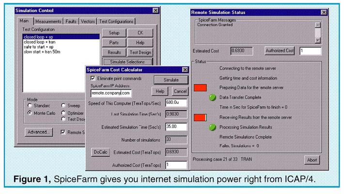
With the release of Design Validator version 8.2.5 and Test Designer version 8.9.5, users will have a new feature in their Simulation Control dialog. The Simulate button will direct the software to run the simulations on a remote "Farm" of computers. Before connecting to a SpiceFarm™, you are required to estimate the cost using the SpiceFarm™ Cost Calculator. Once you have made an estimate and authorized an expenditure which exceeds the calculator cost, you may go ahead and run the simulations. The software will attempt to make a TCP/IP socket connection to the SpiceFarm™ URL or IP address that you have specified. Once the connection is made, the SpiceFarm™ will see if you have the proper authorization, and, if so, it will begin to receive the files and simulation will begin. The simulations will be spun off to the available SpiceFarm™ machines so that many simulations can be performed at the same time. When a SpiceFarm™ is fully built out, you can run 32 simulations at once. As the simulations are being run, SpiceFarm™ will be checking to see if your cost estimates were correct.
|
If a discrepancy appears, SpiceFarm™ will send corrected information, allowing the user to authorize operations. The speed of a computer is then measured in TOPS, Theoretical Operations Per Second, which is the product of clock speed and the number of execution units. For a Pentium II, or Pentium Pro, 3 execution units are used; for a standard Pentium, there are 2. We seed you with 25e12 Tops or 25 Tera Tops at no cost. That comes to 17 hours of computing using a 200MegHz Pentium P5 chip. For Monte Carlo or Failure simulations, the time you spend waiting will be dramatically reduced. You can purchase additional Tera Tops in 100 Tera Tops increments. The tentative charge will be $500 per 100 TeraTops. The file sized for data transfer runs on the order of 30kbytes which can be transferred in 5 or 10 seconds using ISDN bandwidth, or a few milliseconds using your Intranet LAN. If your simulation time is long compared to this transfer time and you do Monte Carlo or multiple failure simulations, then you will get a dramatic speed improvement.
Setting Measurement Tolerances
In the last newsletter, we showed how test sequences can be selected to perform fault isolation. Now we turn to the product acceptance test and show how the same theory can work to increase production yields.
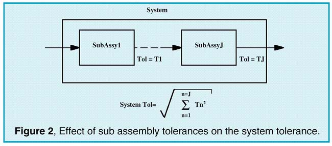
When a system is divided into a number of work packages or subsystems, then the subsystem aggregate tolerance must be equal to the system specification. The generally accepted practice is to root sum square (RSS) the subsystem tolerances. If there were 10 subsystems, each having the same relative complexity, then the tolerance for each subsystem would be the system tolerance divided by the square root of 10.
|
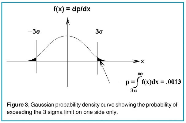
System tolerances are commonly set to the 3 sigma limit; if each subsystem acceptance test was also set for rejection at the 3 sigma limit, then 2 of every 769 subassemblies would be rejected (once at the high limit, and once at the low limit).
|
If you produced a large number of subassemblies, e.g. 10000, then you would have rejected 10000/385*10, or 260 subas-semblies; enough to manufacture 26 systems. If you then built the system without using these rejected units, you would still have substantially the same system level of rejection, because the 1 sigma values would have been altered by only a small amount and thanks to the central limit theorem of probability, the result tends to be Gaussian and is dependent upon the 1 sigma values. So not only would you have rejected the 26 units of subassemblies, you would still have rejected 26 more at the final assembly level.
If you could assure yourself that a subassembly’s performance deviation is only due to part tolerances rather than part failures, then you could approve the subassemblies and take advantage of the tolerance averaging of the system. For $10 billion in sales, you can save $26 million just by choosing the correct tests—and that savings go directly into the bottom line!
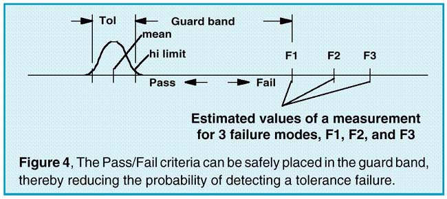
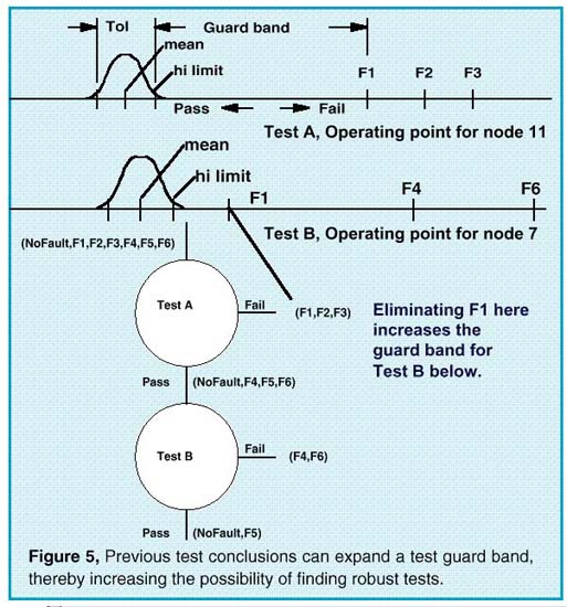
When part failures cause measured values to be substantially outside of the tolerance boundaries, the pass/fail set point can be moved to a much higher sigma value. We call this difference between the expected tolerance limits and the closest failure a "guard band" — it’s safe to put the pass/fail limit within the guard band. Test engineers have long used this observation to their advantage by adding a small fudge factor to test limits in order to eliminate the possibility of rejecting good hardware.
|
If the guard band can be estimated, then you could rationalize this procedure and improve production yield. To get a handle on the guard band, it is necessary to analyze the effect of each possible failure on each candidate measurement. This requires a failure model for each part. Moreover, the size of the guard band will depend upon the possible failure modes for a given test. For example, suppose all prior tests have logically eliminated all but one failure mode. Then the remaining measurement candidates need only consider that one remaining failure mode. Choosing a test sequence that takes advantage of this property results in finding even more tests that have a suitable guard band.
 |
It may seem to be a tall order to estimate the effect of all failures on each candidate measurement; however, using automation techniques coupled with extensive storage of failure results, that is exactly what can be accomplished. The ability to separate test limits from performance limits gives a clear advantage in producing quality electronics using modestly priced test equipment. With the reasonably certain knowledge that no defective parts exist in the delivered system, customers are reassured that fault tolerant designs will perform to high standards. To see how it’s done, ask for an Intusoft Demo CD or download the Test Designer demo from our web site.
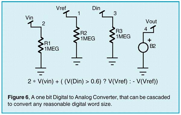
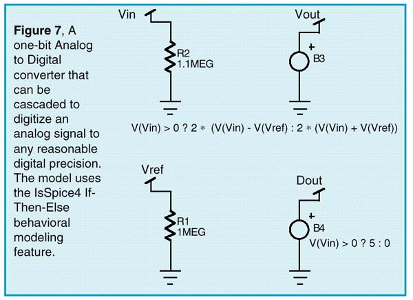
For the purpose of system simulation, many Analog-to-Digital Converters (ADC’s) and Digital-to-Analog Converters (DAC’s) can be modeled using the IsSpice4 B element. The trick in making a generic converter is to first develop a one bit converter that can be cascaded in order to make converters of any reasonable bit length. Rather than basing the conversion algorithm on the sequential successive approximation technique which is widely used for hardware, a pipelined-parallel technique will be used. To make each stage identical, the propagating signal is doubled for each stage. Each element has a reference and signal input, and a propagating output. The DAC output is the input plus twice the reference. The ADC output is twice the input plus/minus the reference, where the plus/minus decision is made to drive the output towards zero. These two one-bit converters are illustrated in Figures 6 and 7.
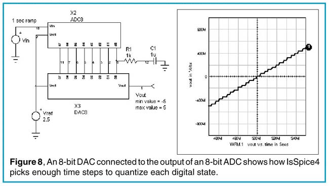
Cascading these one-bit converters to produce an 8-bit conversion is illustrated next in Figure 8. Since these models have nothing to integrate, the time step must either be set manually
|
 |
using Tmax, or additional circuitry must be added to allow the simulator to pick a time step. The series RC connected to the Least Significant Bit (LSB) of the conversion is preferred and sufficient to let the simulator pick the time step automatically.
Since the ADC uses +/- Vref, it produces a result that is the 2’s complement conversion if the sign bit is inverted and one is
|
added to the result. Inverting the sign bit is easy, and adding one can be accomplished by offsetting the analog input. The analog offset is actually 1/2 bit to center the conversion about the quantizing range. Physical realization of these converters produces a very fast pipelined architecture in which the conversion rate is the per stage delay and the pipeline delay time is the stage delay times the number of bits. Fairly low cost conversion of video bandwidth data is possible using this method.
These converters were developed using the ICAP/4 hierarchical schematic feature, and were then made into subcircuits. You can download everything you need to place these models in your libraries by connecting to our web site and selecting the Newsletter #53 button on the front page.
Inverters And Buffers With Smooth Transitions
Digital circuits are sometimes used to produce analog results. For example, feedback around inverters is used to make amplifiers and oscillators. While node bridges can convert between analog and digital, the result is not efficient in terms of using simulator resources, and the infinite gain of the digital models prohibits utilization as amplifiers. A fairly simple generic inverter or buffer can be made to provide a smooth transition that converges easily and simulates the finite gain property of a digital gate. This is accomplished using a cosine tapered gain curve in the transition region coupled with the if-then-else syntax to make a piecewise linear transfer function. Since the model is analog, it will convert to digital using an automatically generated node bridge when the output is connected to a digital input.
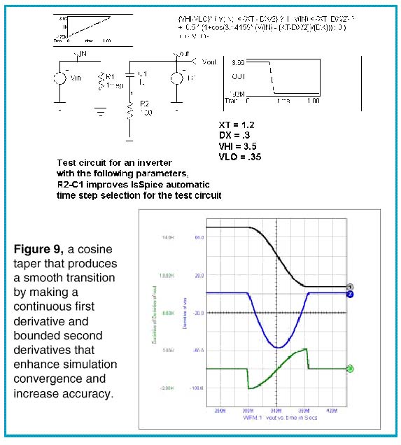 |
Next, a simple oscillator that is commonly used as an internal clock in many IC’s is shown in Figure 10. The first inverter is given a sharper transition to account for the use of several gates in series.
 |
A variation of the inverter is the Hanning window. Hanning windows are applied to time varying signals in order to smooth abrupt changes prior to performing a discrete transform such as a Fast Fourier Transform (FFT). Discrete transforms view data as periodic about their transform interval so that any discontinuities between the beginning and ending values will be spread into the frequency domain. Windowing functions force the value at the beginning and end to be identical. The Hanning window uses a cosine taper to accomplish this task.
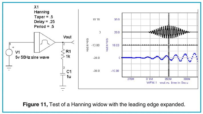
|
The B element description for this window uses a window of the form (1-cos) for the beginning of the period and (1+cos) for the end. The IsSpice4 if-then-else syntax, borrowed from the "C" programming language, is used to piece the various functions together as shown in the following listing.
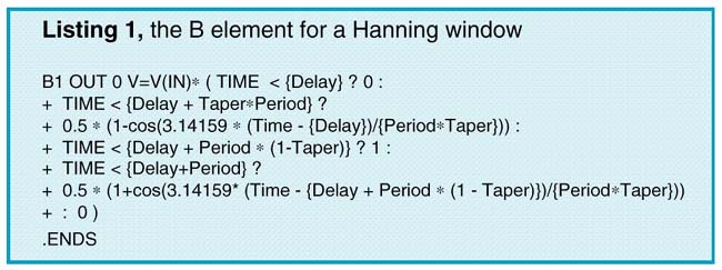
|
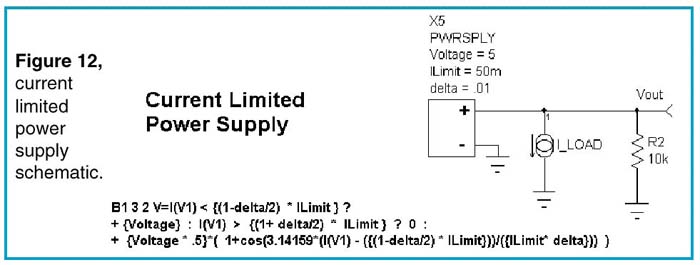
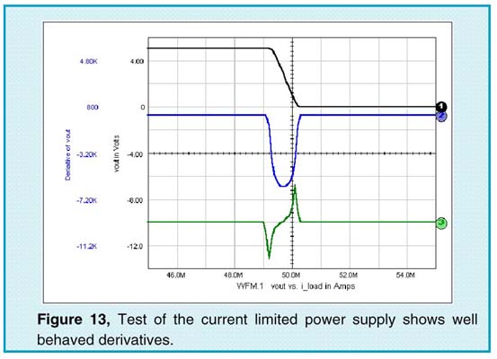
Current limited power supplies are required to test circuits. Using the cosine taper allows a smooth and controlled transition, as illustrated in Figure 13. The sharpness of the transition is controlled by delta; the threshold and low current voltage are also parameters.
|
 |
Initializing Circuits Without UIC
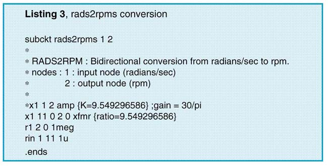
The problem of initialization is a recurring theme in the Intusoft Newsletter. The UIC capability for transient simulations is very convenient; however, it applies globally to everything that’s being simulated. System simulations use subcircuit models for operational amplifiers and other components. Even if these models have a UIC capability, it could put your circuit in the wrong state. Initializing an inductor current, for example, requires the driver transistor to be "ON" and if the transistor is connected to an opamp output, then how is the opamp to know it’s connected to an NPN or PNP circuit? The solution is to NOT use UIC for system level models. You can get around these problems by letting IsSpice4 compute the initial conditions. For an initial inductor current, you simply use a pulse current source that transitions from the initial value to zero at the beginning of the simulation. There are more complex cases in which computation of a pulse voltage or current is difficult. An example would be the initialization of a motor to 100 RPM when you don’t know exactly how it’s connected. In this case, you need to connect a switch between the load and an initializing RPM or voltage. The problem may be complicated further by a model that uses rad/sec, requiring you to supply a units conversion. Moreover, care must be taken when initializing motor speed after beginning the transient simulation because a sufficiently complex simulation would account for the strain caused by the motor acceleration and jerk.
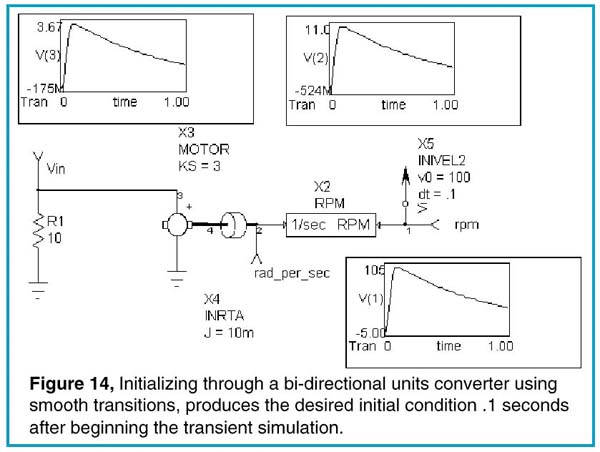
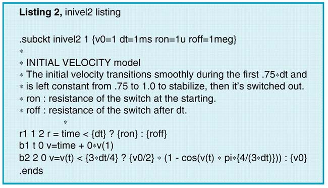
The following example solves all of these problems using a bidirectional units converter and a smooth transitioning source to "slowly" establish the initial condition. Bidirectional conversion conserves power/energy across its boundary. Electrical engineers encounter this most frequently in transformers and power converters or pulse width modulators. When we extend IsSpice4 to mechanical systems, the bidirectional process is also seen in motors and gears. Using bidirectional conversion to convert from one system of units to another, for example, converting rad/sec to RPM has the advantage of being able to initialize a system in a more familiar regime. As we have seen before, the cosine shaped transition limits the acceleration and jerk (first and second derivatives).
Interestingly, the "inivel2" subcircuit (Listing 2) doesn’t really care what units it’s initializing; it could be anything that is represented by a node voltage including velocity, angular velocity, pressure, etc.
|
|
|
Intusoft will release the 8.x.5 ICAP/4 Windows update in May. These items highlight what will be included in the release.
Features:
· New Common Simulation Data Format (CSDF) save option, located in the Simulation Setup dialog under the Save Data button, saves noninterpolated simulation results to a file. It works for the AC, DC, and Transient analyses. The data is saved as the simulation runs (at each time point). This file is readable by Viewlogic’s Viewtrace, and OrCAD’s Probe programs, and in the future, IntuScope. CSDF is useful for long simulations and in the event of a crash or job abort, all of the data will be saved up until the point when the simulation is terminated.
· Update Cache function, located in the Parts menu and in the X Parts Browser dialog, scans the current configuration and creates a list of all of the models, subcircuits, and symbols that are out-of-date, i.e. are different from those contained in the library (.LIB) and symbol (.SYM) files. One or all of the parts can be updated to the latest version. Also listed are part models which are in use but are not in the library database.
· All Simulator IsSpice4 Simulator Options are now available in the Simulation Setup Dialog and its Options Subdialog. The additional options are located under the More button.
· A status button has been added to the Simulation Control dialog for Test Designer. This button allows you to run a subset of the total number of failure analysis simulations. Status also indicates whether each simulation has been run already, not completed or failed.
· ICAPs SpiceFarm, Remote SPICE checkbox - A check box, called Remote SPICE has been added to the Simulation Control Dialog. It allows simulations to be sent over the Internet to a specific IP address (default=Intusoft’s SPICE farm) for execution. If Remote SPICE is checked, a SpiceFarm Cost Calculator is displayed when the Simulate Selections button is selected. The calculator computes the expected simulation cost. The simulation(s) are then run on the SpiceFarm computers. The SpiceFarm may be used for single simulations, Monte Carlo, Optimizer, Failure, and Test Designer simulations (any mode selection). It is available in the Design Validator and Test Designer products.
· Web Help from within SpiceNet is a new Help menu item. Intusoft on the Web was added to the Help menu. It provides access to technical support and the Intusoft home page. The submenu is expandable; users can add their own web links to the submenu.
Enhancements:
· Recently placed parts are appended to the Preferred Parts list.
· SpiceNet remembers the last directory from which a drawing was opened.
· ICAPs support long filenames, long path names, and filenames which contain spaces.
· Subcircuits with parameters work even if no empty curly braces are on the X calling line.
· Win95 Window/Printer sizes of greater than 12 inches (large monitors/large format printers) are allowed.
· A Simulation Setup configuration can be duplicated based onan existing configuration. See the Simulation Setup/Edit button, then the New button.
· Cross-probing memory limit was increased by a factor of 10 to correct cross-probing problems on large waveforms.
· Improved error checking and error messages for invalid B-element syntax and parameter passing.
· Edit symbols directly from the Parts Browser via the new Edit Symbol button. The Parts Browser now displays the path to the symbol and library for the selected part.
· The Find function in the browser is activated simply by typing when the Parts Browser dialog is displayed.
· Part-based help has been added to the part Property help.
· Digital source plugin for 1 to 32 bit bus, including specialized stimulus support;also added a Laplace plugin.
· Added approximately 1000 new models.
· Enhanced Sensitivity data in the IsSpice4 output file.
· Support for Hierarchical parameter passing. Improved support for PSpice ©; parameter passing syntax.
Free Web Calculator and IBIS-2-SPICE Converter
Intusoft offers free software utilities and useful downloads on its web site (http://www.intusoft.com). A new Units Converter/ Calculator and an IBIS-to-SPICE converter are now posted; other free items (SPICE evaluation versions, models, technical articles, and application notes) are on the web page also.
The Units Calculator is a novel program that converts between various types of quantities, i.e. distance (inch, foot yard, mile, meters), energy (erg, joule, ft-pound), force (dyne, newton, pounds), and pressure (millibar, bar, pascal, mm Hg). It also evaluates sequences of mathematical expressions. It is programmable - users may add their own unit conversions and constants. The calculator supports trigonometric, transcendental, and many common math operations.
The IBIS-to-SPICE converter translates IBIS (I/O Buffer Information Specification) data sheet information into SPICE models and supports IBIS versions 1.1, 2.1, and 3.0. It is extensible and allows various SPICE model syntax variations and topologies to be programmed. It reads and parses the IBIS data sheet and extracts the appropriate data tables, pin parasitics, package parasitics, etc. and merges the data into a model template file, yielding a SPICE subcircuit. The default model template is for Intusoft’s IsSpice4 syntax; templates can be constructed for other simulators in order to accommodate the variety of behavioral SPICE syntax used by different SPICE programs. The converter generates models for the multiple pins and signals that may be included in a single IBIS data sheet, and can also extract typical, best or worse case models.
8.X.6 - More Bang for the Buck
A new product release is scheduled for September, 1998. Design Validator and SALT will join the ICAP/4 Deluxe package, along with both Power and RF libraries - a big value that only adds a small change to the existing package price. It comes FREE with maintenance. Plus, users will receive the SpiceFarm capability.
In addition, Monte Carlo becomes scripted. IsSpice4’s Interactive Control Language (ICL) will be added, allowing computationally intensive problems to be offloaded to the SpiceFarm. Test Designer will receive SALT. SpiceFarm will gain a T1 interface and software which enables users to run multiple machines over their company’s Intranet.
Newsletters Page | Issue 54 | Issue 53 | Issue 52 | Issue 51 | Issue 50
©2002 Copyright Intusoft, All Rights Reserved.