| Newsletter List | |
|
|
|
|
Intusoft is excited to release its latest ICAP/4 8.x.11 software this summer. Over the past several months a dedicated technical team has put forth an unprecedented effort to provide valuable extensions to the existing ICAP/4 2450 build. The first of these capabilities stems from an intense modeling effort, assembled from the engineering community’s custom modeling requests. Many of the devices were very complex in nature. To the surprise of the requestors, the devices were successfully modeled, and with a very high level of accuracy. ICs such as sophisticated PWMs, regulators, and specialized operational amplifiers were amongst the list. Discrete devices included select Schottky diodes, an extensive collection of saturable magnetic cores to Magnetics Designer, and special power MOSFETs. Even a solar cell/panel was added to the ever-growing IsSpice4 model collection, which now totals more than 1,000 new full custom devices since the free service began a year ago. Several unique generic models have also been added, enabling the engineer to easily tweak inherent modeling parameters to create unique versions of ICAP/4’s newest op-amps, UJTs, SCRs, and power MOSFETs. |
|
||||||||||||
The new generic models provide something no other SPICE tool furnishes – the ability to quickly create custom models from several different types of generic components, over and above the usual BJT, op-amp, diode, etc. The generic representations, of course, can also be used as is. Further, SpiceMod now accommodates new advanced N and P channel power MOSFETs. This adds to its existing provision of 15 different types of discrete component models, easily created from datasheet entry. A major notable change is that ICAPS can now generates a new .PAR file to help users better understand and debug complex designs. This file consists of two sections. In the first section, all parameters defined in the top level of the design, and all default parameters defined in every subckt in the design, are listed with their values. In the second section, all passed parameters to every instance of every subckt in the design are listed along with the computed values of the parameters. This file is used in complex design (e.g. heirarchical drawings, multiple nesting of subckts, passed parameters with expressions) to confirm that the correct values are passed for every instance of a subckt. |
|||||||||||||
|
|
Many requests have been made for nonlinear core models, particularly for the SPICE models that come from the Magnetics Designer software. Magnetics Designer has some nonlinear parameters available internally, so that it’s possible to make an accurate model for many cores. The powdered cores, in particular, are valuable candidates for automated models. Adding the extra complexity to the model is generally unnecessary if a design doesn’t near saturation. The saturation limits can be computed and an alarm set to warn of potential problems. However, some designs allow the core to enter saturation with the circuit itself limiting the stress. Peak current-limit pulse width modulators are among this kind of circuit. The approach taken for the new Magnetics Designer update is to allow the user to select from a number of different models, including the existing linear model. These core models have also been included in cores.lib that is distributed with the power supply library, and the newsletter subscription. Pressing the new Core Select button in the IsSpice tab brings up the Spice Core Model Select dialog shown in Figure 1.
|
|||||
|
|||||
|
Before going on to describe construction of saturable core models, here’s a few useful simulation techniques used in deriving the new models. You can get a lot of extra mileage from your simulator by running DC sweeps. Here are a couple of tricks. First, when the data tends to be spaced uniformly in a log plot, then the sweep variable can be expanded using an exponential function. Then when the log is taken, the data point will be spaced uniformly. If you don’t use this trick, you need to set the sweep step very small to resolve the data for larger x-axis values. That causes too much unnecessary data for smaller x-axis values. The sweep generator model in our library does this by setting
The sweep variable then ranges from 0 to 1. Example:
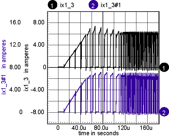
Next, the u-H plot can be obtained by differentiating the B-H plot. The differentiation in the model uses an inductor to differentiate current and feed it back as a voltage. But that process requires time domain or frequency domain analysis. A simple DC sweep with post-simulation differentiation achieves the same objective, and with a lot less computational effort. Figure 3 illustrates the result. 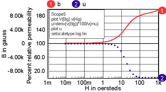
|
|||||||||||||||||||||||||||||||||||||||||||||||||||||||||||||||||||||||||||||||||||||
| |
|||||||||||||||||||||||||||||||||||||||||||||||||||||||||||||||||||||||||||||||||||||
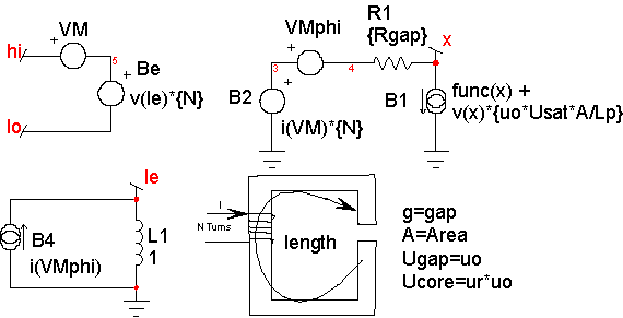
Magnetic cores are described by their B-H loop properties. Inductance is proportional to the permeability, which is proportional to the derivative or slope of B with respect to H. A typical B-H curve and permeability-H curve is shown in Figure 5. For most of our discussion, hysteresis will be ignored; it can be shown that the area enclosed by the hysteresis curve is proportional to core loss energy. Moreover, the loss increases significantly at higher frequencies. Placing a resistor, Rcore, across the nonlinear inductor accurately models the high-frequency loss. Hysteresis will appear in the B-H curve if the current used to compute H includes the current delivered to the combination of the resistor and the nonlinear inductor. 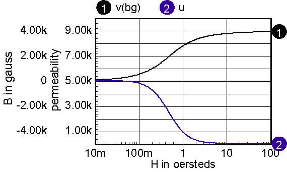
Accurate modeling of inductance requires a good estimate of the permeability-H characteristic. Then the function in the model, func(x) in Figure 4, is formed by integrating the permeability curve. Inductors are made by using a magnetic material in combination with an air-gap. The gap can be introduced as a discrete gap or as a distributed gap. The most common way of making a distributed gap is by mixing non-magnetic filler with powdered magnetic material. Discrete gaps are made by inserting a dimensionally stable material, such a paper, between the core pieces. The inductor’s core can be modeled using a table, or by finding continuous functions that approximate the B-H characteristics. Continuous functions are less susceptible to discontinuities, and as a result they should work better in a simulator. When using a table model, the most commonly available data is from a B-H curve. Inaccuracies in transcribing the data from a data sheet curve to a table will result in magnifying the error in the permeability function (that’s because permeability is the derivative of the B-H curve). The B-H curves must be carefully filtered and their derivatives tested to assure a stable simulation. On the other hand, continuous functions can be fit to permeability-H curves using optimization techniques. Errors in transcribing data are reduced statistically, and because the continuous functions tend to describe the device physics. Many data sheets give what appear to be valid continuous functions as the ratio of polynomials. The problem with this approach is that the polynomial ratio departs from physical reality outside the region where data was used to make the best fit. This shortcoming is illustrated in Figure 6. It also illustrates how easy it is to use the IntuScope waveform viewer to evaluate and plot equations. 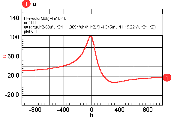
Powdered cores exhibit a larger swing in H for the same percentage change in permeability. The reason for this is because the powdered particles will saturate first where they are almost touching each other, slowly increasing the air gap as the magnetic material saturates. Solid cores with a single gap tend to saturate uniformly so that the permeability drops more rapidly. The packing arrangements and shape of the powdered particles vary, based on the manufacturing process. The solution of Maxwell’s equations in a closed form function is unknown, even for simple packing geometry. We will get around this problem by examining several reluctance models based on four generic solutions. Continuous functions for permeability are useful for defining the
The 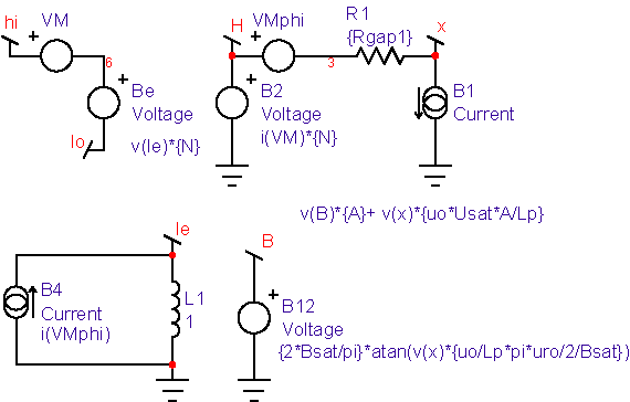
Notice that the permeability curves, for example Figure 5, look very much like magnitude vs. frequency plots. When the slope of log(permeability)/log(H) is an integer multiple of 20db/decade, then an even polynomial ratio can be used to describe the curve, and in theory an integral can be found. Note: the restriction on even values arises from the symmetry of permeability for negative MMF-
Notice that it retains the even symmetry, but its slope for
and for H=0,
solving for a, we fine a=1, and k1 = uro
Unlike the atan function, this one grows to infinity. But the slope drops below 1, the permeability of free space. We can therefore define
and from 5.1 with
Notice that for all of the models, a Usat term is added in the B1 current (Flux analog) source. Usat is usually set to 1, the relative permeability of free space. It may become convenient to give it a larger value to fit data for very high magnetic fields. The next shape is the sigmoid B-H curve. It’s extremely sharp and can be used for square-loop material such as Orthonal or Permalloy. Starting from the B-H curve, the sigmoid is defined as:
and finally
Figure 9 shows the competed model. 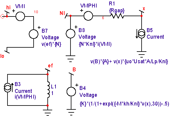
Notice that this model contains a scaling parameter, Kni. It’s used to reduce the voltage that represents the MMF at node NI to normalize the voltage range, so that the VSECTOL convergence option gives good results. It’s usually set to kh, conveniently making the voltage at node NI equal to H in Oersteds. Yet another B-H loop comes from combining a linear relation below a field, Then an exponential function is used thereafter such that the inductance at where This exponential model is used internally in Magnetics Designer for the reluctance model used to compute inductance verses current. It provides a reasonably accurate model for powdered cores; however, there is an abrupt change in the derivative of inductance where the two functions are joined, as seen in Figure 10. It predicts sharper cutoff characteristics for Ferrite cores. 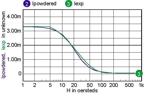
Figure 11 illustrates the differences for a gaped core. 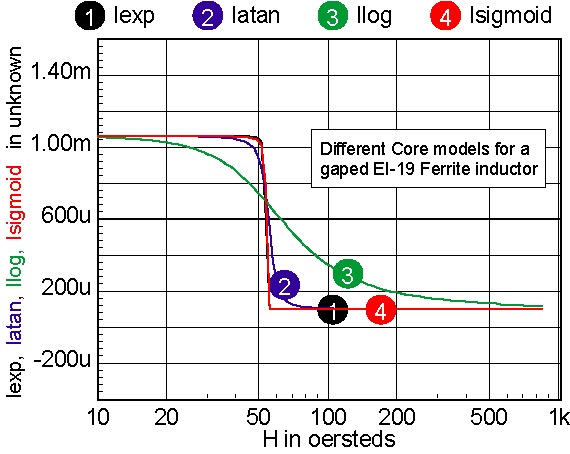
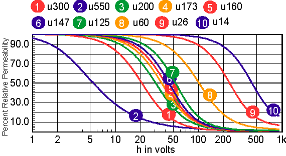
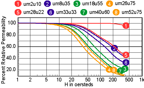
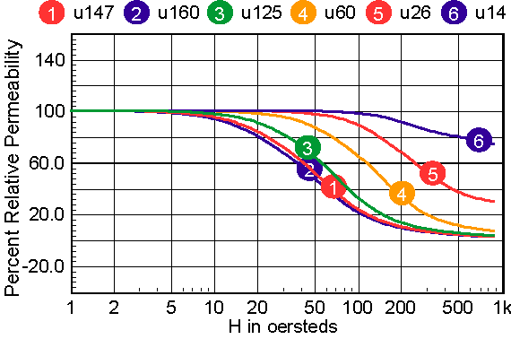
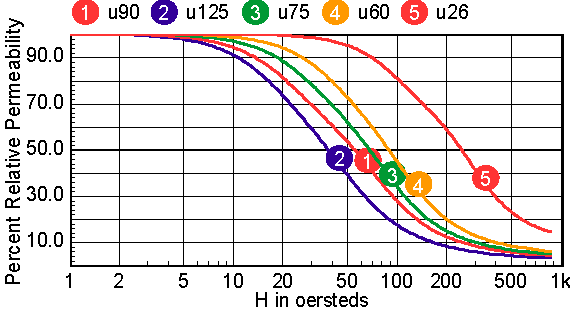
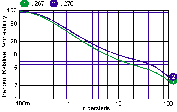
For cores that have distributed gaps, such as MPP or Kool Mu powered cores, a special reluctance model is used. In general, two cores are made in parallel, each with its own gap. The mix parameter tells how much the first core contributes to the H=0 permeability. Note: parallel cores correspond to series inductors. Table 2 shows the combination of free parameters used to get the best fit to the published Table 2: parameters for powdered cores The RMS error is in general based on data for percent initial permeability = 80,50,20. When these permeability values can’t be achieved, three different values are substituted. The accuracy to which the charts can be read is larger than the error in the curve fit. Moreover, the initial permeability tolerance is much greater than the curve fit tolerance. Most inaccuracy occurs for percent permeability below 10%, or for deep saturation. Figures 12-16 show the percent permeability verses H for the families in the above table. It is recommended that the atan model be used for other ferrite cores, and the sigmoid model selected for solid cores. Provisions are made for making your own user models, and connecting them to the Magnetics Designer SPICE model. All of the non-linear models use the IsSpice4 syntax and need to be translated if you use another simulator.
|
|||||||||||||||||||||||||||||||||||||||||||||||||||||||||||||||||||||||||||||||||||||
|